Table of contents
Note: Jeff Donahue, Philipp Krähenbühl and Trevor Darrell at Berkeley published a paper independently from us on the same idea, which they call Bidirectional GAN, or BiGAN. You should also check out their awesome work at https://arxiv.org/abs/1605.09782.
What is ALI?
The adversarially learned inference (ALI) model is a deep directed generative model which jointly learns a generation network and an inference network using an adversarial process. This model constitutes a novel approach to integrating efficient inference with the generative adversarial networks (GAN) framework.
What makes ALI unique is that unlike other approaches to learning inference in deep directed generative models (like variational autoencoders (VAEs)), the objective function involves no explicit reconstruction loop. Instead of focusing on achieving a pixel-perfect reconstruction, ALI tends to produce believable reconstructions with interesting variations, albeit at the expense of making some mistakes in capturing exact object placement, color, style and (in extreme cases) object identity. This is a good thing, because 1) capacity is not wasted to model trivial factors of variation in the input, and 2) the learned features are more or less invariant to these trivial factors of variation, which is what is expected of good feature learning.
These strenghts are showcased via the semi-supervised learning tasks on SVHN and CIFAR10, where ALI achieves a performance competitive with state-of-the-art.
Quick introduction to GANs
GAN pits two neural networks against each other: a generator network \(G(\mathbf{z})\), and a discriminator network \(D(\mathbf{x})\).
The generator tries to mimic examples from a training dataset, which is sampled from the true data distribution \(q(\mathbf{x})\). It does so by transforming a random source of noise received as input into a synthetic sample.
The discriminator receives a sample, but it is not told where the sample comes from. Its job is to predict whether it is a data sample or a synthetic sample.
The discriminator is trained to make accurate predictions, and the generator is trained to output samples that fool the discriminator into thinking they came from the data distribution.

To better understand GANs, it is necessary to describe it using a probabilistic framework. Two marginal distributions are defined:
- the data marginal \(q(\mathbf{x})\), and
- the model marginal \(p(\mathbf{x}) = \int p(\mathbf{z}) p(\mathbf{x} \mid \mathbf{z}) d\mathbf{z}\).
The generator operates by sampling \(\mathbf{z} \sim p(\mathbf{z})\) and then sampling \(\mathbf{x} \sim p(\mathbf{x} \mid \mathbf{z})\). The discriminator receives either the generator sample or \(\mathbf{x} \sim q(\mathbf{x})\) and outputs the probability that its input was sampled from \(q(\mathbf{x})\).

The adversarial game played between the discriminator and the generator is formalized by the following value function:
On one hand, the discriminator is trained to maximize the probability of correctly classifying data samples and synthetic samples. On the other hand, the generator is trained to produce samples that fool the discriminator, i.e. that are unlikely to be synthetic according to the discriminator.
It can be shown that for a fixed generator, the optimal discriminator is
and that given an optimal discriminator, minimizing the value function with respect to the generator parameters is equivalent to minimizing the Jensen-Shannon divergence between \(p(\mathbf{x})\) and \(q(\mathbf{x})\).
In other words, as training progresses, the generator produces synthetic samples that look more and more like the training data.
Learning inference
Even though GANs are pretty good at producing realistic-looking synthetic samples, they lack something very important: the ability to do inference.
Inference can loosely be defined as the answer to the following question:
Given \(\mathbf{x}\), what \(\mathbf{z}\) is likely to have produced it?
This question is exactly what ALI is equipped to answer.
ALI augments GAN’s generator with an additional network. This network receives a data sample as input and produces a synthetic \(\mathbf{z}\) as output.
Expressed in probabilistic terms, ALI defines two joint distributions:
- the encoder joint \(q(\mathbf{x}, \mathbf{z}) = q(\mathbf{x}) q(\mathbf{z} \mid \mathbf{x})\), and
- the decoder joint \(p(\mathbf{x}, \mathbf{z}) = p(\mathbf{z}) p(\mathbf{x} \mid \mathbf{z})\).
ALI also modifies the discriminator’s goal. Rather than examining \(\mathbf{x}\) samples marginally, it now receives joint pairs \((\mathbf{x}, \mathbf{z})\) as input and must predict whether they come from the encoder joint or the decoder joint.
Like before, the generator is trained to fool the discriminator, but this time it can also learn \(q(\mathbf{z} \mid \mathbf{x})\).

The adversarial game played between the discriminator and the generator is formalized by the following value function:
In analogy to GAN, it can be shown that for a fixed generator, the optimal discriminator is
and that given an optimal discriminator, minimizing the value function with respect to the generator parameters is equivalent to minimizing the Jensen-Shannon divergence between \(p(\mathbf{x}, \mathbf{z})\) and \(q(\mathbf{x}, \mathbf{z})\).
Matching the joints also has the effect of matching the marginals (i.e., \(p(\mathbf{x}) \sim q(\mathbf{x})\) and \(p(\mathbf{z}) \sim q(\mathbf{z})\)) as well as the conditionals / posteriors (i.e., \(p(\mathbf{z} \mid \mathbf{x}) \sim q(\mathbf{z} \mid \mathbf{x})\) and \(q(\mathbf{x} \mid \mathbf{z}) \sim p(\mathbf{x} \mid \mathbf{z})\)).
Experimental results
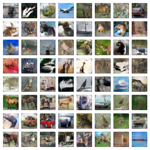
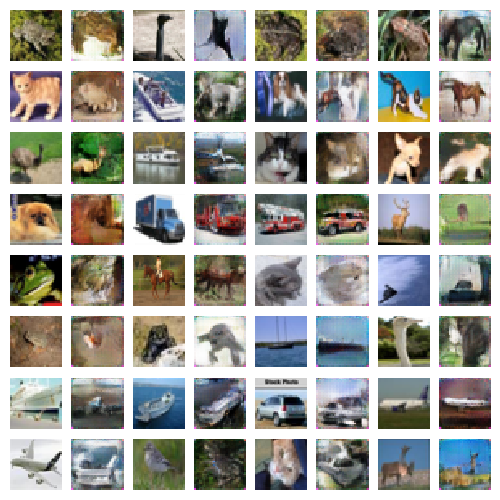
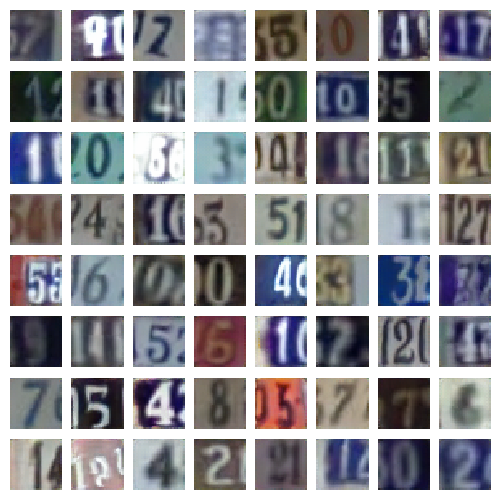
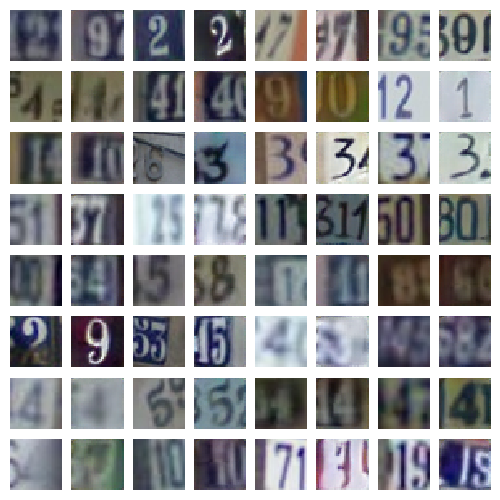
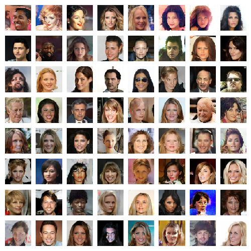
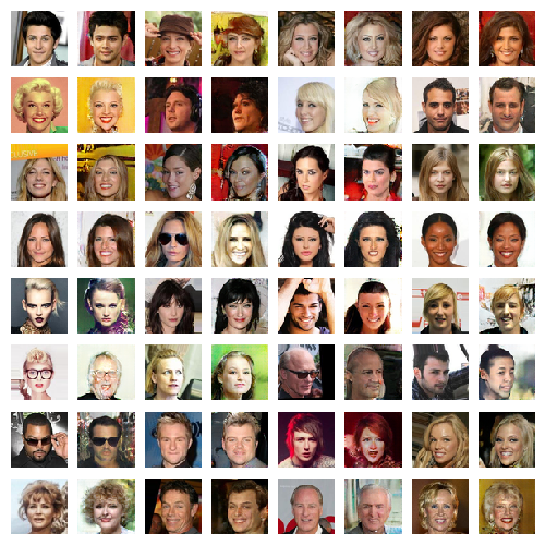
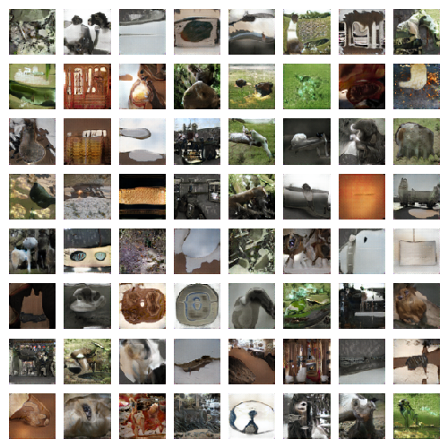
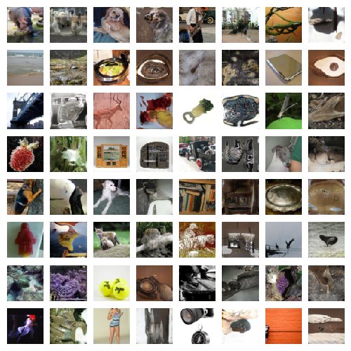
Regarding reconstructions: odd columns are validation set examples, even columns are their corresponding reconstructions (e.g., first column contains validation set examples, second column contains their corresponding reconstruction).
CIFAR10
The CIFAR10 dataset contains 60,000 32x32 colour images in 10 classes.
 |
 |
SVHN
SVHN is a dataset of digit images obtained from house numbers in Google Street View images. It contains over 600,000 labeled examples.
 |
 |
CelebA
CelebA is a dataset of celebrity faces with 40 attribute annotations. It contains over 200,000 labeled examples.
 |
 |
Tiny ImageNet
The Tiny Imagenet dataset is a version of the ILSVRC2012 dataset that has been center-cropped and downsampled to \(64 \times 64\) pixels. It contains over 1,200,000 labeled examples.
 |
 |
Latent space interpolations
As a sanity check for overfitting, we look at latent space interpolations between CelebA validation set examples. We sample pairs of validation set examples \(\mathbf{x}_1\) and \(\mathbf{x}_2\) and project them into \(\mathbf{z}_1\) and \(\mathbf{z}_2\) by sampling from the encoder. We then linearly interpolate between \(\mathbf{z}_1\) and \(\mathbf{z}_2\) and pass the intermediary points through the decoder to plot the input-space interpolations.
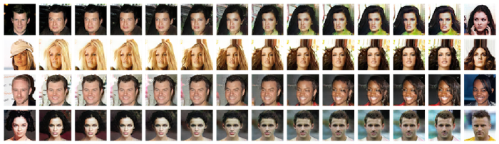
We observe smooth transitions between pairs of example, and intermediary images remain believable. This is an indicator that ALI is not concentrating its probability mass exclusively around training examples, but rather has learned latent features that generalize well.
Conditional generation
ALI can also be used for conditional generative modeling by providing the encoder, decoder and discriminator networks with a conditioning variable \(\mathbf{y}\).
We apply the conditional version of ALI to CelebA using the dataset’s 40 binary attributes. The attributes are linearly embedded in the encoder, decoder and discriminator. We observe how a single element of the latent space z changes with respect to variations in the attributes vector \(\mathbf{y}\).
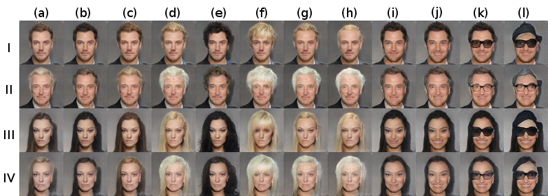
The row attributes are
- I: male, attractive, young
- II: male, attractive, older
- III: female, attractive, young
- IV: female, attractive, older
The column attributes are
- a: unchanged
- b: black hair
- c: brown hair
- d: blond hair
- e: black hair, wavy hair
- f: blond hair, bangs
- g: blond hair, receding hairline
- h: blond hair, balding
- i: black hair, smiling
- j: black hair, smiling, mouth slightly open
- k: black hair, smiling, mouth slightly open, eyeglasses
- l: black hair, smiling, mouth slightly open, eyeglasses, wearing hat
Semi-supervised learning
We investigate the usefulness of the latent representation learned by ALI through semi-supervised benchmarks on SVHN and CIFAR10.
SVHN
| Number of labeled examples | 1000 |
|---|---|
| VAE (M1 + M2) 1 | 36.02 |
| SWWAE with dropout 2 | 23.56 |
| DCGAN + L2-SVM 3 | 22.18 |
| SDGM 4 | 16.61 |
| GAN (feature matching) [^7] | 8.11 ± 1.3 |
| ALI (ours, L2-SVM) | 19.14 ± 0.50 |
| ALI (ours, no feature matching) | 7.42 ± 0.65 |
CIFAR10
| Number of labeled examples | 1000 | 2000 | 4000 | 8000 |
|---|---|---|---|---|
| Ladder network 5 | 20.40 | |||
| CatGAN [^6] | 19.58 | |||
| GAN (feature matching) [^7] | 21.83 ± 2.01 | 19.61 ± 2.09 | 18.63 ± 2.32 | 17.72 ± 1.82 |
| ALI (ours, no feature matching) | 19.98 ± 0.89 | 19.09 ± 0.44 | 17.99 ± 1.62 | 17.05 ± 1.49 |
Discussion
We first compare with GAN on SVHN by following the procedure outlined in Radford et al. (2015) 3. We train an L2-SVM on the learned representations of a model trained on SVHN. The last three hidden layers of the encoder as well as its output are concatenated to form a 8960-dimensional feature vector. A 10,000 example held-out validation set is taken from the training set and is used for model selection. The SVM is trained on 1000 examples taken at random from the remainder of the training set. The test error rate is measured for 100 different SVMs trained on different random 1000-example training sets, and the average error rate is measured along with its standard deviation.
Using ALI’s inference network as opposed to the discriminator to extract features, we achieve a misclassification rate that is roughly 3.00 ± 0.50% lower than reported in Radford et al. (2015) 3, which suggests that ALI’s inference mechanism is beneficial to the semi-supervised learning task.
We then investigate ALI’s performance when label information is taken into account during training. We adapt the discriminative model proposed in Salimans et al. (2016) [^7]. The discriminator takes \(x\) and \(z\) as input and outputs a distribution over \(K + 1\) classes, where \(K\) is the number of categories. When label information is available for \(q(x, z)\) samples, the discriminator is expected to predict the label. When no label information is available, the discriminator is expected to predict \(K + 1\) for \(p(x, z)\) samples and \(k \in \{1,\ldots,K\}\) for \(q(x,z)\) samples.
Interestingly, Salimans et al. (2016) [^7] found that they required an alternative training strategy for the generator where it tries to match first-order statistics in the discriminator’s intermediate activations with respect to the data distribution (they refer to this as feature matching). We found that ALI did not require feature matching to achieve comparable results.
We are still investigating the differences between ALI and GAN with respect to feature matching, but we conjecture that the latent representation learned by ALI is better untangled with respect to the classification task and that it generalizes better.
Comparison with GAN on a toy dataset
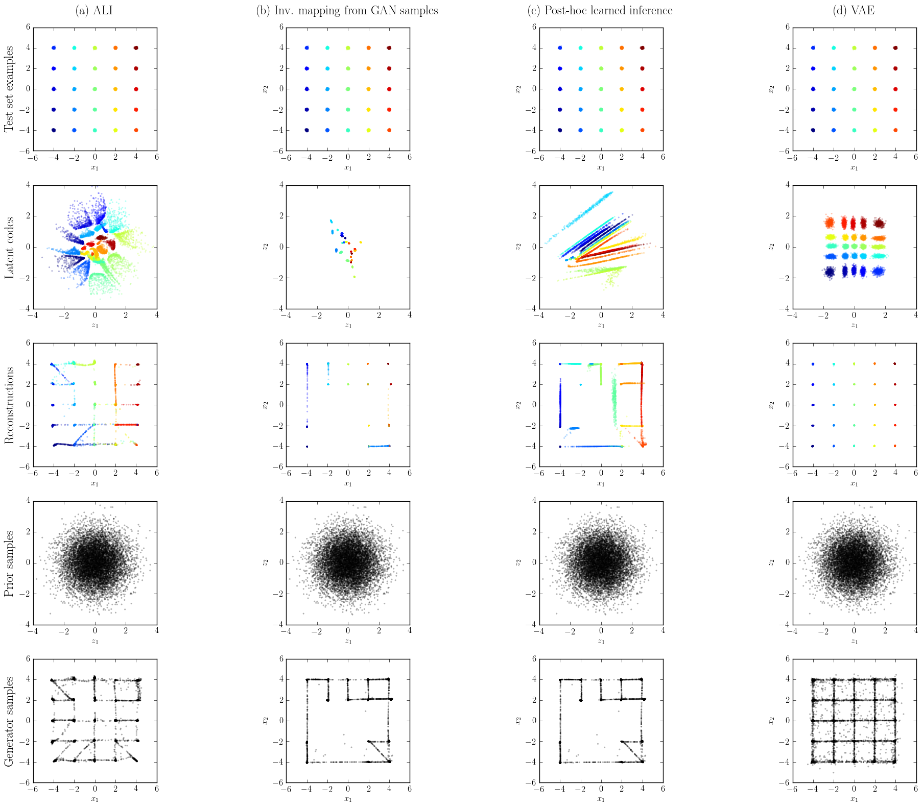
To highlight the role of the inference network during learning, we performed an experiment on a toy dataset for which \(q(x)\) is a 2D gaussian mixture with 25 mixture components laid out on a grid. The covariance matrices and centroids have been chosen such that the distribution exhibits lots of modes separated by large low-probability regions, which makes it a decently hard task despite the 2D nature of the dataset.
We trained ALI and GAN on 100,000 \(q(x)\) samples. The decoder and discriminator architectures are identical between ALI and GAN (except for the input of the discriminator, which receives the concatenation of x and z in the ALI case). Each model was trained 10 times using Adam with random learning rate and \(\beta_1\) values, and the weights were initialized by drawing from a gaussian distribution with a random standard deviation.
We measured the extent to which the trained models covered all 25 modes by drawing 10,000 samples from their \(p(x)\) distribution and assigning each sample to a \(q(x)\) mixture component according to the mixture responsibilities. We defined a dropped mode as one that wasn’t assigned to any sample. Using this definition, we found that ALI models covered 13.4 ± 5.8 modes on average (min: 8, max: 25) while GAN models covered 10.4 ± 9.2 modes on average (min: 1, max: 22).
We then selected the best-covering ALI and GAN models, and the GAN model was augmented with an encoder using the following procedures:
- learned inverse mapping : A mapping from \(x\) to \(z\) is learned from GAN samples. This corresponds to learning an encoder to reconstruct \(z\), i.e. finding an encoder such that \(\mathbb{E}_{z \sim p(z)}[\mid\mid z − G_z(G_x(z))\mid\mid_2^2] \approx 0\). We are not aware of any work that reports results for this approach. This resembles the InfoGAN learning procedure but with a fixed generative model and a factorial Gaussian posterior with a fixed diagonal variance.
- post-hoc learned inference: Training is decomposed into two phases. In the first phase, a GAN is trained normally. In the second phase, the GAN’s decoder is frozen and an encoder is trained following the ALI procedure (i.e., a discriminator taking both \(x\) and \(z\) as input is introduced). In this setting, the encoder and the decoder cannot interact together during training and the encoder must work with whatever the decoder has learned during GAN training.
The encoders learned for GAN inference have the same architecture as ALI’s encoder. We also trained a VAE with the same encoder-decoder architecture as ALI to outline the qualitative differences between ALI and VAE models.
We then compared each model’s inference capabilities by reconstructing 10,000 held-out samples from \(q(x)\) (see figure above). We observe the following:
- The ALI encoder models a marginal distribution \(q(z)\) that matches \(p(z)\) fairly well (row 2, column a). The learned representation does a decent job at clustering and organizing the different mixture components.
- The GAN generator (row 5, columns b-c) has more trouble reaching all the modes than the ALI generator (row 5, column a), even over 10 runs of hyperparameter search.
- Learning an inverse mapping from GAN samples does not work very well: the encoder has trouble covering the prior marginally and the way it clusters mixture components is not very well organized (row 2, column b). Reconstructions suffer from the generator dropping modes.
- Learning inference post-hoc doesn’t work as well as training the encoder and the decoder jointly. It appears that adversarial training benefits from learning inference at training time in terms of mode coverage. This also negatively impacts how the latent space is organized (row 2, column c). However, it appears to be better at matching \(q(z)\) and \(p(z)\) than when inference is learned through inverse mapping from GAN samples.
- Due to the nature of the loss function being optimized, the VAE model covers all modes easily (row 5, column d) and excels at reconstructing data samples (row 3, column d). However, VAEs have a much more pronounced tendency to smear out their probability density (row 5, column d) and leave “holes” in \(q(z)\) (row 2, column d). Note however that recent approaches such as Inverse Autoregressive Flow may be used to improve on this, at the cost of a more complex mathematical framework.
In summary, this experiment provides evidence that adversarial training benefits from learning an inference mechanism jointly with the decoder. Furthermore, it shows that our proposed approach for learning inference in an adversarial setting is superior to the other approaches investigated.
Conclusion
The adversarially learned inference (ALI) model jointly learns a generation network and an inference network using an adversarial process. The model learns mutually coherent inference and generation networks, as exhibited by its reconstructions. The induced latent variable mapping is shown to be useful, achieving results competitive with the state-of-the-art on the semi-supervised SVHN and CIFAR10 tasks.
Processing Systems_. [^6]: Springenberg, J. T. (2015). Unsupervised and semi-supervised learning with categorical generative adversarial networks. arXiv preprint arXiv:1511.06390. [^7]: Salimans, T., Goodfellow, I. J., Zaremba, W., Cheung, V., Radford, A., and Chen, X. (2016). Improved techniques for training GANs. arXiv preprint arXiv:1606.03498.
-
Kingma, D. P., Mohamed, S., Rezende, D. J., and Welling, M. (2014). Semi-supervised learning with deep generative models. In Advances in Neural Information Processing Systems, pages 3581–3589. ↩
-
Zhao, J., Mathieu, M., Goroshin, R., and Lecun, Y. (2015). Stacked what-where auto-encoders. arXiv preprint arXiv:1506.02351. ↩
-
Radford, A., Metz, L., and Chintala, S. (2015). Unsupervised representation learning with deep convolutional generative adversarial networks. arXiv preprint arXiv:1511.06434. ↩ ↩2 ↩3
-
Maaløe, L., Sønderby, C. K., Sønderby, S. K., and Winther, O. (2016). Auxiliary deep generative models. arXiv preprint arXiv:1602.05473. ↩
-
Rasmus, A., Valpola, H., Honkala, M., Berglund, M., and Raiko, T. (2015). Semi-supervised learning with ladder network. In _Advances in Neural Information ↩